Advanced Acourate Digital XO Time Alignment Driver Linearization Walkthrough

In this article, I walk through the steps using Acourate to create a 3-way digital crossover (XO) for tri-amping my speakers. Additionally, using the audio toolbox functions of Acourate, I walk through the steps of time aligning the drivers, linearizing each driver, and performing a final room correction.

With respect to room correction, I recommend reading, “Acourate Digital Room and Loudspeaker Correction Software Walkthrough” for an introduction to Acourate. The article details the steps of acquiring a calibrated microphone, measuring the system, and designing a baseline room correction to provide the listener with a perceptually flat frequency response at the listening position.

My goal is to make this guide repeatable so anyone following the same steps should be able to achieve similar results. Using digital XO, time aligning and linearizing the drivers, and correcting the room’s frequency and excess phase response, increases my systems imaging resolution so my speakers *disappear*.[PRBREAK][/PRBREAK]

The objective measure is called Interaural Coherence Coefficient (IACC) which is a measure of channel and room reflection equality for the first 80 milliseconds of sound travel. IACC is a common standard especially for describing the spaciousness of sound in concert halls. Uli’s innovative use is in the opposite direction, to get a measure of channel and room reflection equality over time.

System Under Test

I am going to briefly describe the components of my system to assist in understanding how Acourate fits in. I have included a picture of my audio system to not only help visualize the components, but to show that my speakers and room are far from perfect. My speaker cabinets have the opposite of rounded edges for diffraction. Not really visible in the picture is that the stereo is offset in the room, where the left speaker is almost in the corner and the right speaker is midway on the long wall. My room has a poor ratio. The stereo offset and room ratio cannot be changed.

On the positive side, I have added bass traps behind the speakers, thick carpet/underlay from speakers to listening position, broadband absorbers on the ceiling, and back wall to help reduce early reflections. I have carefully set up the system as symmetrical as possible given the physical room constraints.

From a system design perspective, I favor full-range, high efficiency, dynamic floor standing speakers driven by Nelson Pass designed Class A amplification. The techniques described here can be applied to virtually any system that can be bi-amped or tri-amped.

The speaker kit is a Bob Crites designed Cornscala Type C, which uses the same bass reflex enclosure as the Klipsch Cornwall (PDF), but with a 15” custom designed Klipsch clone woofer. Midrange: Selenium D405 (PDF) compression driver and 2380A horn. Treble: Selenium D220Ti compression driver and HM11-25 horn. Custom 500 Hz/5000 Hz passive XO. Aside from disconnecting the passive XO and wiring in additional speaker terminals, I replaced the high frequency compression drivers with a pair of BMS 4540 about six months ago as these drivers have frequency extension to 30 kHz.

The amplification is Nelson Pass DIY A40 stereo Class A amplifier that drives the 97 dB @ 1w/1m sensitivity 15” 4 ohm woofers and 4 x DIY Amp Camp Amp’s (ACA) single-ended Class A Mosfet amplifiers drive the 110 dB and 114 dB @ 1w/1m sensitivity midrange and high frequency compression drivers respectively. While the ACA’s are rated at 6 watts, with the sensitivity of the compression driver/horn combos, I very rarely push 1 watt into them.

It’s the woofers that require the power, and compared to the compression drivers, this sets the upper SPL limit of the system. With the passive XO, Bob Crites measured system efficiency to be 100 dB @ 1w/1m. At 10 watts that would be 110 dB SPL and sound twice as loud as perceived by my ears. 100 watts = 120 dB = threshold of pain or 4 times as loud relative to 1 watt. I have ~80 watts Class A stereo on tap (with 260,000 micro-farads of power supply reservoir capacitance) for the woofers, so estimate around 117 dB max SPL. That is way more SPL than I would ever listen to in a home environment and it’s nowhere near the maximum power rating of any of the drivers. Conversely, at the other extreme, the speakers sound full-range and dynamic, even listening at 65 dB SPL.

The A/D D/A Converter is a Lynx Hilo which is a two channel converter, but is flexible enough to be configured for 6 D/A channels, with level trim on the analog outputs to the mid and high frequency amplifiers. This allows me to level balance the higher sensitivity compression drivers to the lower sensitivity woofer and bass reflex cabinet combo.

The computer audio music player is JRiver MC 19 in which I use its built-in 64-bit Convolution engine to host the Acourate designed FIR filter. The FIR filter contains the 3-way linearized XO’s, time alignment adjustments, and room (frequency and excess phase) correction. The stereo music played through JRiver is convolved in real-time with the Acourate designed FIR correction filters and outputs 6 digital channels. These channels are routed through Lynx Hilo’s digital patch system to the appropriate analog outputs (with level trim for mids and highs) which are plugged directly into the inputs of the 6 amplifiers. Volume is controlled digitally (with volume protection) by JRiver.

With the brief “system under test” description out of the way, let’s get started. The high level steps are:

1. Create a 3-way digital XO, measure the system, perform an intermediate room correction, report IACC and listening results.
2. Time align the drivers in each cabinet, measure the system to verify time alignment, perform an intermediate room correction, report IACC and listening results.
3. Linearize each driver by measuring 30cm on axis to each driver, check distortion characteristics, and measure the linearized drivers for verification.
4. Perform final room correction using the time aligned and linearized XO’s, report IACC and listening results.

Digital XO

The sonic benefits of bi and tri-amplification are well documented. However, with the advent of massive personal computing power, coupled with the power of sophisticated audio DSP software like Acourate, we can create virtually any digital XO we desire at high resolution (64 bits). I recommend reading Dr. Uli Brueggemann's (author of Acourate) paper entitled, “Thoughts on Crossovers” (PDF).

Digital XO enables driver time alignment, and linearizing each individual driver, with the goal of increasing the systems IACC.

I am ready to create my first Digital XO. Again, I recommend reading the introduction article to become familiar with working with Acourate, setting up work spaces, etc., as I will not be covering these procedures here.

Launch Acourate:

From the Generate Menu, select Crossover:

As described in Uli’s Digital XO article, there are several XO filter types to choose from. In my case, I am selecting the default Neville-Thiele, 2nd order filter and entering in the same XO corner frequencies as my passive XO’s of 500 Hz and 5000 Hz:

Click Calculate and Save:

If I look in the Acourate workspace directory, I see the generated XO files:

Now load up the left side 3-way XO’s in Acourate. Remember, each time a file is to be loaded, make sure the appropriate active curve radio button is selected. For the 3 XO files here, I selected radio buttons 1, 2, and 3 before loading each curve:

This is what the XO’s look like when loaded into Acourate. Looking at amplitude:

Here are a couple of ways to view the digital XO’s to get familiar with what is happening. When the amplitude scaling in the time domain chart is set to Auto one can view/unview each curve by the according checkbox in the chart legend.

See how the amplitude in the chart is changing when XO3 is unselected and then XO2. The lowpass filter has a pretty small amplitude compared to the highpass filter, but the frequency response chart has the same level 0 dB for all crossovers. I did not include the individual pics for this as it is best to unselect interactively with the software so one can see the level changes in the time chart. It is a worthwhile exercise as later in the article we will need to locate the pulse peaks for each driver in order to time align the drivers.

One can add the three crossovers by using TD-Functions - Addition into an empty curve (series):

The result is a perfect Dirac pulse in the time domain:

See how the XO’s amplitudes sum together in the frequency domain:

Perfect.

Acourate crossovers (and correction filters) are generated in the sequence 1L, 1R, 2L, 2R, 3L, 3R. This means bass left, bass right, midrange left, midrange right, tweeter left, and tweeter right.

Next step is to generate a multiway wav file that contains the XO’s to be used in the measurement. Under the File menu, select Save Multiway Filter WAV:

Here I select XO1L96.dbl. The save dialog appears, give it a name to indicate a multiway filter:

Click save. Now from the LogSweep Menu, select LogSweep Recorder:

It is assumed that one knows how to load the mic cal.wav file from the introduction to Acourate article. Clicking in the Filter field will open a dialog box. Choose the multiway wav filter that contains the XO’s that were just saved. The label should now display a 6 channel filter.

The LogSweep Recorder will use 6 continuous channels starting with the first selected output channel in ascending order. E.g. if output channel 1 is selected, then the speaker drivers have to be connected by
output1 = bass left, output 2 = bass right, output 3 = midrange left, output 4 = midrange right, output 5 = tweeter left, output 6 = tweeter right.

Of course one can change the physical connections and use the routing capabilities of a soundcard or converter mixer. But the logical channels will follow the same principle. The LogSweep Recorder will automatically play a left and right sweep in the correct channel sequence.

The resulting pulse responses for left and right channel will contain the recorded signals of all 6 drivers.

Before clicking on Start Recording, ensure that the output level is at a reasonable level. Also check that the sweep start and end cover the desired frequency range. In my case, I am sweeping from 10 Hz to 30 kHz with a 96 kHz sample rate. However, best practice is to use a 48 kHz sample rate and sweep to 24 kHz (i.e. 10 Hz to 24 kHz).

Click Start Recording. Once the recording is finished, both PulseL96 and PulseR96 will be displayed:

The intermediate step here is to produce a Room Correction as per the introduction to Acourate article, have a seat, and listen to the results. I am not going to walk through the room correction process here as I am saving that for the final correction. But one does need to know how to configure JRiver’s Output and Convolver, and prepare a configuration filter file format for referencing the FIR filters in order to listen to the intermediate room correction.

Configure JRiver for 6 output channels:

Configure JRiver’s Convolver to host the FIR filter config file:

Here is a link to the description of cfg file format and an example cfg file that can be downloaded.

If one follows the room correction procedure in the introduction to Acourate article, the last step is to run a Test Convolution. Here is the result of the measured and corrected IACC:

Note the overall IACC values. From a listening perspective, and I am not good with subjective descriptions, I hear the benefits of active XO’s as linked to earlier. The sound remains crystal clear as the volume increases with no hint of dynamic range compression or distortion. When I had the passive XO in place, and with the A40 amp cranked up, there is enough current to make it buzz euphonically.

With a baseline digital XO and room correction in place, proceed to time aligning the acoustic centers of the drivers in each speaker cabinet.

Time Alignment

If one took the time to examine the digital XO’s in the time domain, as described in the XO section, it would have been noted the different amplitude peak levels for each XO. The high frequency XO being the highest amplitude and the low frequency XO the lowest. When looking at the impulse response of a speaker system, most folks look at the peak, which is usually the tweeter’s peak and does not necessarily include the bass or midrange peak, especially if the system is not time aligned.

To help find each peak in the time domain for each driver, I am going to create another XO, but this time with an artificial delay built in. The idea is that if each driver is separated by a known delayed amount, it will be easier to pick out the pulse of each driver and determine if the drivers are time aligned or not.

For example, I am going to delay the midrange by 1000 samples and the tweeter by 2000 samples. If the tweeter and midrange were aligned perfectly with the bass driver, I would measure the midrange exactly 1000 samples behind the bass driver, and tweeter 1000 samples behind the midrange.

As a side note, every time a sweep is made using the LogSweep Recorder and displayed in the time domain chart, the software finds the highest peak amplitude (i.e. the tweeter) and sets the peak at sample 6000 on the time domain chart. It is important to keep this in mind for the following procedure.

In a separate workspace, generate another XO in Acourate, same XO values as before, but note the added delay of 1000 samples in the midrange XO (Delay 2 = 1000) and 2000 samples in treble XO (Delay 3 = 2000):

Click Calculate and Save. As before, under the File menu, select Save as multiway WAV and load this into the LogSweep Recorder:

Start Recording. Once finished, what I want to do is load the left pulse that I just measured along with the 3 “original” left XO’s (i.e. the ones with no delay) into Acourate. The non-time delayed XO’s are going to be my visual “helpers” to find the pulse peaks for the woofer and midrange driver. Should look something like this:

Now for some math. The originally generated XO’s are linear phase filters, so the peaks are at the midway point of the total number of samples. 65,536 taps divided by 2 = sample position 32768 is where the XO peaks are located.

The tweeter in Pulse96 (that I just measured with the delayed XO’s) is located at sample 6000. It is the highest red peak towards the left side of the time chart. Remember for every sweep, the highest peak (i.e. the tweeter) is automatically set to sample 6000.

With treble XO selected as the active curve, using TD-Functions, select Rotation. What I want to do is rotate XO3 by -26768 samples (i.e. 32768 – 6000) for comparison. We use the – sign to indicate rotation to the left. Another way to think of rotation is time or distance. The resolution is 1 sample. So, 1/96000 = .01 milliseconds. In distance that is .343 centimeters or 0.135”. After clicking Rotate Signal:

Now select active curve XO2 and rotate by -27768 (i.e. 32768 – 6000 + the 1000 sample artificial delay). Then select active curve XO1 and rotate by -28768 (i.e. 32768 – 6000 + the 2000 sample artificial delay). Clicking on the Time radio button displays:

As mentioned previously, if the tweeter and midrange were aligned perfectly with the bass driver, I would see the midrange exactly 1000 samples behind the bass driver, and tweeter 1000 samples behind the midrange.

To find the bass driver pulse peak, we use XO1 as the visual “helper” to assist in locating the peak. Unselect XO2 and XO3 in the chart legend. Using the markers, zoom in around 3000 to 6000 sample range. Given the low level amplitude of the bass driver, one will also have to turn the Auto amplitude check boxes off and enter in smaller values in order to see the bass pulse peak. Check and uncheck XO1 to ensure that the bass peak is being located:

The green curve is XO1 and the red curve is the bass pulse peak. Ensuring that I have selected Active Curve 1, (i.e. Pulse96L), I can set the left and right markers on either side of the pulse and read the MaxM sample number (highlighted top right in the chart below) which automatically detects the pulse peak for the bass driver:

The bass peak is at sample 4030. Also note the positive polarity of the signal. This is a good way to check each individual driver’s polarity.

Following the same procedure as above, but now with XO2, locate the midrange peak. Again, one may have to check and uncheck XO2 to be sure it is the midrange peak being located and adjust the chart amplitude numbers accordingly:

The green display is XO2 and the red display is the midrange peak. Setting the markers again, and looking at the MaxM number highlighted to the right of the chart, the midrange driver peak occurs at sample 5060.

Therefore the distance between tweeter and bass is not 2000 samples, but 1970 samples (i.e. 6000 – 4030). The distance between midrange and tweeter is not 1000 samples, but 940 samples (i.e. 6000 – 5060). Therefore the tweeter is too quick. Or put another way, the acoustic center of the tweeter is before the acoustic center of the midrange and bass. In fact, all 3 drivers are not acoustically aligned. I repeated the same procedure for the right channel, and the delays measured the same.

If I delay the tweeter by 30 samples, that lines up with the artificial distance to the bass of 2000 samples (i.e. 1970 + 30 = 2000). If I delay the tweeter by another 30 samples (60 samples total) and the bass also by 30 samples, then it all lines up to the midrange. In other words, the bass needs to be delayed by 30 samples and the tweeter by 60 samples to line up with the acoustic center of the midrange driver.

To do this, create another workspace and generate new XO’s without any delays. Then open up both the left and right XO1 (bass) and rotate each one to the right by 30 samples (TD-Functions – Rotation). Save each one (overwrite) with the same name. Now open up left and right XO3 (treble) and rotate each one to the right by 60 samples and save each. Read this paragraph again to be sure of the procedure. It is easy to make changes to the wrong XO or not save one.

Another way to do this is rotate XO1 (bass) to the left -30 and XO2 (midrange) rotation to the left by -60 to line up with the tweeter, instead of the midrange as described in procedure above. In the end, this produces the same result as above, but keeps the tweeter XO peak at 32768. This may be an easier way to understand and makes it easier to verify the time alignment as the tweeter is always referenced at sample 6000.

Whichever way is chosen, the next step is to create and save the multiway WAV file and load the new time aligned XO into the LogSweep Recorder and take another measurement.

However, if one wishes to verify the time alignment results first, create another XO, this time with the Delay 2 = 1000 and Delay 3 = 2000. Then rotate the appropriate XO’s by the values obtained above. Create and Save the multiway WAV filter, load into LogSweep Recorder and take another measurement. Using the same procedure as before to locate the peaks (more rotations), one can verify that the midrange is exactly 1000 samples behind the bass driver and tweeter exactly 1000 samples behind the midrange. I verified in my system that this is the case.

Once verified, use the new XO’s, with the correct delays (i.e. in my case bass delayed by 30 samples and tweeter by 60), and re-measure the system and use those new measures to perform another intermediate room correction. Again, refer to the introduction to Acourate article for the room correction procedure:

After following the room correction procedure, and generating the Test Convolution, here is the IACC:

Time aligning the driver’s results in an incremental improvement over the previous IACC values.

Subjectively speaking, I was surprised at how much time alignment made an audible difference. Probably exacerbated by the fact it is a 3-way system and none of the drivers were aligned. The audible difference can be described in two ways.

The depth of field of the stereo image (or soundstage or soundscape) appears to resolve to infinity behind the speakers. Another way of putting it is point source sound. I have listened to a few time aligned speakers and monitors over the years and was always impressed by their capability to resolve depth of field.

But what really surprised me was the tone quality of the speakers changed, for the better. There was something about my system that did not sound quite right tonally. Even after tri-amping, it was still there, and I thought it would go away as my first suspicion was the drivers were operating outside their linear range of operation as the passive XO is only 6 dB per octave. But that wasn’t it.

However, once the system was time aligned, the tone quality issue I heard is now gone. I suspect my ears are sensitive to the tweeter arriving first as it always had a forward sounding tone quality, no matter how it was eq’d. Whatever the cause, those minor tonal issues are now absent.

Driver Linearization

The idea is to measure each driver, in my case, tweeter, midrange, and woofer, in the near field. Near field meaning positioning the mic on axis to each driver 30cm away.

It is always good to check the behavior of the drivers by examining their distortion characteristics. We want to see if the driver’s distortion is linear over its operating range as the driver could possibly exhibit anomalies near the XO frequencies and may require adjusting the XO corner frequency.

I will start with the left tweeter first. Looking up the specs for the BMS 4540 compression driver that I linked to in the system description earlier, it states that its frequency operating range is from 1200 Hz to 30 kHz. So that’s what I used as the sweep range in the LogSweep Recorder:

Careful, with respect to output volume and the channels that the LogSweep Recorder is routed to. For example, what I don’t want to do is sweep the tweeter full range (i.e. sweep start = 10Hz) as that will likely damage the tweeter. Always double check before start recording. Also note to leave the mic in the same position as the procedure is to check the distortion, linearize the driver with the XO, and then check the result of the linearization, then move on to the next driver.

Start recording. Here is the result of the recording after I deleted the right sweep as I am only interested in the left tweeter at this time:

In this first section of these steps, I am going to walk through how to extract and view the distortion characteristics.

Copy the files: \MyDocuments\Acourate\Logsweep\Logsweep96_rec.wav and Inverse96.dbl into the workspace folder because the recording always gets overwritten with each new recording. I renamed the files to add Left in front of the name of the file, so I do not overwrite anything as I continue with the procedure.

Under the Edit menu, clear all curves. Under the LogSweep menu, select LogSweep Convolution *without* pulse extraction. Set result curve to Series 1:

The LogSweep measurement file is named: LeftLogSweep96_rec.wav and the LogSweep inverse file is named: LeftInverse96.dbl.

Now switch to the time domain chart:

Select the main peak in the time domain chart using the left and right markers:

Under the LogSweep menu, select Extract pulses and harmonic distortion. Check the logsweep parameters to make sure it matches the sweep range started out with:

Click Extract Pulse and Distortion:

What is displayed is the basic pulse response plus 4 series with distortion k2 to k5. The distortion is sample rate converted. So a k2 distortion bump at e.g. 1 kHz can be compared to k1 at 1 kHz (indeed the distortion is at 2 kHz). In the case of the BMS 4540 compression driver, looks good with no anomalies across its operating range, plus no issues at the XO frequency I have selected (e.g. 5 kHz.). While I did not calibrate the level, one can always look up the distortion by converting dB to percent distortion. If interested and want to review the details later, one can save all 6 curves.

The next steps of this procedure is to linearize the tweeter. Again, leaving the mic in its original position as the tweeter will need to be swept again to verify the linearization.

From the Edit menu, clear all curves.

Load the pulse – in this case LeftPulse96

Apply TD-Functions - Frequency Dependent Windowing: 15/15, 15/15 cycles before/behind the pulse peak. Select Series 2 as the result curve:

Click Calc sliding window:

Set the markers to frequencies 2570 Hz and 24627 Hz. At this position the smooth curve has peaks, so I am interested in linearizing this range and discarding the rest:

Apply TD-Function - Phase Extraction - minphase - below 2570, above 24627. Note my markers are off a bit, but it’s not critical to be identical:

Apply FD-Function - Amplitude Inversion – minphase:

Click Calculate Inversion:

Zoom in on amplitude a bit for a closer view.

Before then next step, ensure that Active Curve radio button 5 has been selected, otherwise the existing curve will be overwritten and will have to start over again.

Load the crossover XO3L96 that I actually use into active curve 5. Actual XO meaning the time aligned XO that was prepared in the time alignment procedure.

Apply TD-Function - Convolution of Inverse and XO:

Click Convolution:

Before the next step, select Active Curve radio button 2 and clear curve from under the edit menu as I do not require this anymore and need space for another curve. Once Curve 2 has been cleared, make sure that Curve 6 radio button is selected as the active curve to apply the next function.

Optional: If one switches on File – Expert Mode, I can save the result of a calculation in any of the series and thus overwrite an existing curve. This makes the handling of a lot of curves sometimes easier.

Apply TD-Function - CutNWindow - length 65536, start position 0, no windowing:

Click Cut’N Window:

Uncheck the display of all curves except the original XO and the CutNWdw.

Apply TD-Function - Normalization - individual gain. This sets the max gain to 0 dB:

Click Normalize:

Save the linearized XO (i.e. CutNWdw active curve 2) as the new XO3L96.

Now re-measure the tweeter with the new linearized XO in place to verify the result. To do that, clear all curves, open up the new XO .dbl file, and save as a mono wav file to load into the LogSweep Recorder:

Launch the LogSweep Recorder and load the XO mono wav file. Make sure the frequency sweep range, output level, and channel routing is the same as started with at the top of the procedure:

Start recording.

The green curve is the original measure and the red curve is the measurement verification after linearization within the XO range. Zoomed in view to get the picture:

Note these are full resolution displays, no smoothing has been applied.

Went from ±6.5 dB to ±1 dB response within the tweeter XO range at 30 cm. distance.

The idea is to repeat this procedure for each individual driver, in my case 5 more drivers. Patience is a virtue.

There is some contention as to whether the bass drivers should be linearized due to the wavelengths involved. There is no doubt going to be some room interaction. However, in my case, it turns out the IACC increased with the bass drivers linearized as opposed to not linearized. If you are following the procedure, go ahead and measure and linearize the bass drivers.

Linearizing the midrange driver, using the frequency range from the spec sheet (i.e. 300 Hz to 7 kHz), went from ±7 dB over the frequency range and the linearized measure is ±2 dB. Again a significant improvement.

Same improvement for the woofer. Rather than showing each individual drivers distortion and measurement result, here are the before and after driver linearization results for the left side at 30cm distance on axis for each driver.

Before:

After:

Again, full resolution displays with no smoothing. The right side is virtually identical in both response and distortion characteristics. As it turns out, I did not have to adjust any XO corner frequencies. However, I may experiment by lowering the bass to midrange corner frequency.

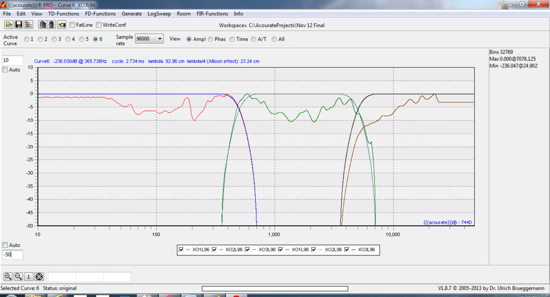
Here are the regular XO’s compared with the linearized XO’s, left side:

Final Room Correction

At this stage, I have created the digital XO, time aligned, and linearized all drivers. Referring to the introduction article on Acourate, I used the exact same room correction steps and parameters in this article for consistency and being able to compare.

It is presumed that one has already saved the final XO’s, created the multiway wav filter, loaded the filter in the LogSweep Recorder (along with the mic cal file), and taken a measurement at the listening position. Here is the result of my measurement, looking at the amplitude response and zoomed in a bit:

Under the Room menu, select Room Macro 1: Amplitude Preparation:

I feel it is worth pointing out that Uli’s measurement analysis uses a proprietary frequency dependent windowing (FDW) algorithm. Having used several acoustical analysis software packages over the years, to my ears, Acourate represents best what I see on the charts compared to what I perceive with my ears. The FDW is long at low frequencies (100’s of milliseconds) and short at high frequencies (< a millisecond). I recommend Ackcheng’s site for technical details as it is an important concept to understand.

Run Macro 1: Amplitude Preparation:

While I was able to get flat frequency response from the drivers at a distance of 30 cm, I can see the effects of the room on the response in the low end at a distance of just over 3 meters to the listening position. Easily taken care of by the room correction. Above 1 kHz, the response is already ±2 dB to 28 kHz.

Select Room Macro 2: Target Curve Design:

As mentioned in the introduction article on Acourate, it is very important to get the target curve flat to 1 kHz, and using 1 kHz as a hinge point, make a straight line to -6 dB at 20 kHz. This target design represents a perceptually flat frequency response at the listening position.

One may have to zoom in to be sure, because as little as .1 dB off will make an audible difference as the straight slope covers a broad frequency range from 1 kHz to 20 kHz. Save target as target.dbl.

An alternative way, which I use, is to prepare a text file with pairs of frequency and amplitude:

100 0

1000 0

20000 -6

Then File – Import Amplitude…, save as target.dbl, and use that in the next step. It is worth the extra time to get the target specification exact.

Run Room Macro 3: Inversion:

Run Room Macro 4: Filter Generation:

Note that the Excess Phase window also uses frequency dependent windowing. Here is more information on pre-ringing compensation.

I hope folks understand that with frequency dependent windowing of both amplitude and excess phase, and a FIR filter length of 65,536 samples, why the bass response in this listening position still sounds even.

In fact, the bass response sounds even no matter where I listen in the room.

To check the proposed room correction, run Room Macro 5: Test Convolution. Here is the IACC:

The process of linearizing the drivers has made a significant impact on improving the IACC from the previous values.

Here I am looking at the frequency response with frequency dependent windowing applied (i.e. Room Macro 1: Amplitude Preparation) on the correction:

Note the vertical amplitude scale. Other than a couple ±2 dB swings, the response is ±1 dB from 32 Hz to 2 kHz and ±0.5 dB from 2 kHz to 28 kHz within the perceptually flat target response. Equally important is how closely the two channels are identical to each other.

Step response in the time domain:

For further points on step response and other Acourate technical thoughts, refer to Ackcheng’s excellent site. CA readers may also be interested in reading about Tony Knight’s system.

Conclusion

Replacing the passive XO with Acourate digital XO, time aligning and linearizing all drivers, and applying room correction, has significantly (audibly and measurably) increased the tone quality and imaging resolution of my system. With the grills on the speakers, no one would believe it is a horn based system.

To try and relate what this means, allow me to share a short story. Over 40 years of listening to music on audio systems, 10 of those as a recording/mixing and live sound engineer, I can’t count the number of systems/environments I have heard – hundreds. But I do remember the best sounding system/environment being a studio in Vancouver, Canada, where no expense was spared for the acoustic design and gear. I was there from the ground up studio and control room build, to paying customers using the facility. I learned a lot about the acoustic design of a state of the art recording and mixing studio.

Listening to this state of the art system/control room at first is a bit startling as it does give the real sense of envelopment, like I was actually sitting in the studio at the mic position and having the studio sound envelop around me. Setting up a stereo pair of mics in the studio, the control room monitors disappear and one gets a real sense of being *in* the studio as opposed to listening *to* the studio. It is the closest representation I have heard compared to physically being in the same space as the musicians.

In addition to the reflection free zone (RFZ), and properly diffused room decay, the acoustic design of this control room had no parallel surfaces, and literally one half of the control room is an exact mirror image of the other half. The purpose being is to make the left and right channels response as identical as possible, over a finite period of time. Subjectively, this is what makes speakers “disappear” and all one is left with is the sound image.

Uli achieves similar results through the use of high resolution (64 bit) digital signal processing in his Acourate software where each channel and room reflections are tuned as close to identical over a defined time period. The objective measure is called IACC. I have shown by using Digital XO, driver time alignment and linearization, and room correction all contribute to increasing my systems IACC.

Please note that an average setup results in an IACC around 75% based on Uli’s experience. Higher IACC values, like what I have obtained (88.5% and 87%), does require very careful setup and consideration to room design, as I have outlined in the system under test section.

Using Uli’s designed FIR correction filters, I get that same sense of envelopment and being immersed in the sound as compared to the state of the art system/control room mentioned above. For example, the song Chaiyya Chaiyya has a vibrato synth or string effect that slowly sweeps from one channel to the other. This sound extends well beyond the left and right physical location of the speakers. One gets the sense that it reaches all the way to the listening position and is directly perpendicular to the left and right ears as the effect sweeps. The sense of envelopment, image height, width, and depth of field feels like being in the music.

The Live Cream Album at Royal Albert Hall is an excellent live recording that has a stereo pair at the house mix position, in addition to the stage mics. One can really hear the envelopment of the Hall. Jack Bruce’s bass guitar and vocals on Spoonful sound staggeringly huge with the Albert Hall reverb. Listening to the image size of Cream in Royal Albert Hall belies the actual physical size of my listening room, and not in an exaggerated way either. The feeling is like being in the recorded music’s acoustic space. I never thought I would hear that in my living room.

Acourate optimizes my system to reproduce the music as close as possible to the content of the recording. Highly recommended!

Thanks to Bob Sutcliffe who took the photos of my system.

Enjoy being in the music!

About the author

Mitch “Mitchco” Barnett

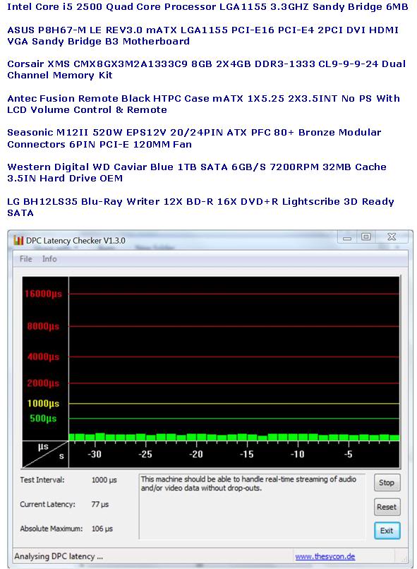
I love music and audio. I grew up with music around me as my Mom was a piano player (swing) and my Dad was an audiophile (jazz). At that time Heathkit was big and my Dad and I built several of their audio kits. Electronics was my first career and my hobby was building speakers, amps, preamps, etc., and I still DIY today . I also mixed live sound for a variety of bands, which led to an opportunity to work full-time in a 24 track recording studio. Over 10 years, I recorded, mixed, and sometimes produced over 30 albums, 100 jingles, and several audio for video post productions in a number of recording studios in Western Canada. This was during a time when analog was going digital and I worked in the first 48 track all digital studio in Canada. Along the way, I partnered with some like-minded audiophile friends, and opened up an acoustic consulting and manufacturing company. I purchased a TEF acoustics analysis computer which was a revolution in acoustic measuring as it was the first time sound could be measured in 3 dimensions. My interest in software development drove me back to University and I have been designing and developing software ever since.